🧮 Lab 3 — Introduction to Queuing Theory & Java Modelling Tools (JMT)
Duration: ~1 hour
Environment: Windows, Linux, or macOS (JMT is Java-based)
🎯 Learning Objectives
- Understand the basic components of a queuing system (arrivals, service, queues, customers).
- Learn to use the Java Modelling Tools (JMT) suite.
- Build, simulate, and analyze simple queuing networks.
- Compare system metrics: utilization, throughput, average queue length, response time.
⚙️ Setup Instructions
- Download JMT: https://jmt.sourceforge.net/
- Requires Java (≥ JDK 8)
- Unzip and run
JSIMgraph.jar(for simulation models)
Tools Overview
| Tool | Description |
|---|---|
| JSIMgraph | Build and simulate queuing network models |
| JMVA | Analyze models analytically |
| JABA | Build models programmatically in Java |
🧩 Part 0 — Quick Recap: Queuing Theory Basics
Key Symbols:
- λ (lambda) = arrival rate (customers per second)
- μ (mu) = service rate (customers served per second)
- ρ (rho) = utilization = λ / μ
For M/M/1 queue:
- Average number in system: L = ρ / (1 − ρ)
- Average waiting time: W = 1 / (μ − λ)
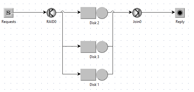
🧩 Example 1 — RAID-0 style Parallel I/O (Fork–Join)
A request is split across k disks and the reply is sent after all parts finish (synchronous join). RAID (Redundant Array of Independent Disks) is a data storage technology that combines multiple physical disks into a single logical unit to improve performance, fault tolerance, or both. Different RAID levels (e.g., RAID 0, 1, 5) determine how data is split, mirrored, or parity-protected across the disks.
🧠 Learning outcomes
By the end of this exercise, students should:
- Understand the concept of fork–join synchronization in queuing networks.
- Observe that variability (heavy tail) in response time increases with more parallel disks.
⚙️ Model overview
| Element | Description |
|---|---|
| Source | Generates incoming I/O requests (arrival rate λ). |
| Fork | Splits each request into k sub-tasks (1 per disk). |
| Disks | Modeled as queueing stations with hyperexponential service times. |
| Join | Waits for all k sub-tasks to finish before reassembling the request. |
| Sink | Collects completed requests. |
Step-By-Step Instructions
Step 1. Create a new model
- Open JSIMgraph → click File → New Model.
- From the toolbar, drag a Source, Fork, Join, k Queueing Stations, and a Sink node onto the canvas.
- Connect them in this order:
- Source → Fork → (Disk1, Disk2, Disk3, …) → Join → Sink
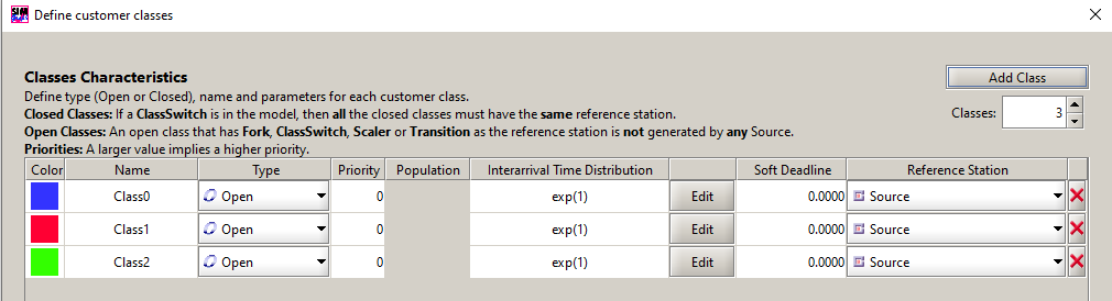
Step 2. Create a Class
- Define distribution (e.g., exponentital, hperexponential etc). Choose λ, mean.
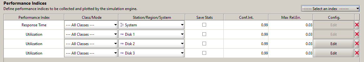
Step 3. Define Performance Indeces (what you want to measure)
Step 4. Run the simulation
🧩 Example 2 — Load Balancer Policies per Class
A router (LB) dispatches to a pool of servers. Compare Random, Round-Robin, and Shortest-Queue (SQ). Use two customer classes with different SLAs.
⚙️ Model overview
| Element | Description |
|---|---|
| Source | Generates incoming I/O requests (arrival rate λ). |
| Router | Dispatches requests to servers. |
| Servers | Modeled as queueing stations |
| Sink | Collects completed requests. |
Step-By-Step Instructions
Step 1. Create a new model
- Open JSIMgraph → click File → New Model.
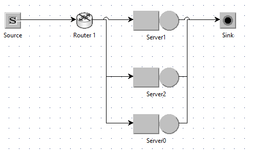
- From the toolbar, drag a Source, Router, k Queueing Stations, and a Sink node onto the canvas.
- Connect them in this order:
- Source → Router → (Server1, Server1, Server1, …) → Sink
Step 2. Create Classes representing different type of requests
- Define distribution (e.g., exponentital). Choose λ, mean.
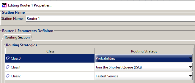
Step 3. Define Routing Strategies for each class
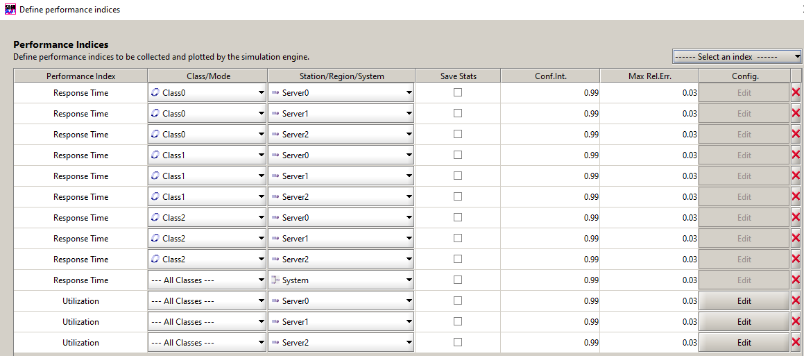
Step 3. Define Performance Indeces (what you want to measure)
Step 4. Run the simulation
🧩 Example - Middleware Node with Prioritization and Network Link
🎯 Goal
In this experiment, we model a middleware system that receives messages of two types—High-priority (alerts) and Low-priority (telemetry)—and forwards them across a shared network link.
We want to study how priority scheduling and message filtering affect throughput and response time for each class.
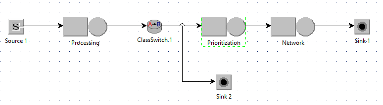
- Processing: models message parsing or validation
- ClassSwitch: filters 20% of Low messages
- Prioritization: optional lightweight classification stage
- NetworkLink: single-server queue representing the network; uses class-based priority scheduling
- Sink: collects transmitted messages
- DropSink: collects filtered-out Low messages
⚙️ Model Configuration
| Parameter | High Priority | Low Priority | Description |
|---|---|---|---|
| Arrival rate (λ) | 2 msg/s | 8 msg/s | Incoming traffic intensity |
| Processing time | 0.020 s | 0.020 s | Exponential (shared CPU) |
| Filtering probability | 1.0 | 0.8 keep / 0.2 drop | Implemented via ClassSwitch |
| Prioritization delay | 0.001 s | 0.001 s | Deterministic |
| NetworkLink service time | 0.008 s | 0.032 s | Deterministic (based on packet size) |
| Scheduling policy | Priority (non-preemptive) | — | High = 1 (highest), Low = 2 |
📊 Performance Indices to Collect
For both classes and the system:
- Throughput [msg/s]
- Response time [s]
- Utilization [%] (of Processing and NetworkLink)
- Number of customers [msg] in queue and in service
- Drop rate [%] for Low messages (from DropSink throughput)
🔬 Experiments to Perform
-
Baseline scenario
- λ_H = 2/s, λ_L = 8/s
- Measure throughput and response times.
- Observe how High messages experience consistently low delay.
-
Increased load
- Increase both arrival rates (e.g., λ_H = 5/s, λ_L = 20/s).
- Observe queue buildup at NetworkLink.
- High messages still get through quickly; Low messages queue longer or drop.
-
Remove filtering
- Change Low’s filtering probability to 1.0 (no drops).
- Compare new response times—expect larger delays due to congestion.
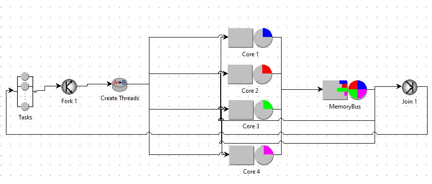
⚙️ Example 5 — Parallel Multicore and Multithreaded Server
🎯 Goal
In this advanced example, we model a parallel server that executes multithreaded tasks on multiple CPU cores, all sharing a common memory bus.
This setup represents a multicore processor where threads run concurrently but contend for shared memory bandwidth.
The goal is to evaluate the scalability of the system and observe how resource contention limits performance.
🧩 System Architecture
Tasks → Fork (Create threads) → ([Core 1] [Core 2] [Core 3] [Core 4]) → MemoryBus →Join
Each job (user request) is decomposed into multiple threads, which are processed on different cores.
All threads share a single MemoryBus before synchronizing at the Join node.
⚙️ Model Configuration
🧠 Workload
| Parameter | Value | Description |
|---|---|---|
| Workload type | Closed classes | Fixed number |
| Population (N) | 10 | Active jobs in the system |
🧩 Routing Configuration
| From → To | Probability | Notes |
|---|---|---|
| Task of type 1 to Core 1 | 1.0 | Pin thread to Core 1 |
| Task of type 2 to Core 2 | 1.0 | Pin thread to Core 2 |
| Task of type 3 to Core 3 | 1.0 | Pin thread to Core 3 |
| Task of type 4 to Core 4 | 1.0 | Pin thread to Core 4 |